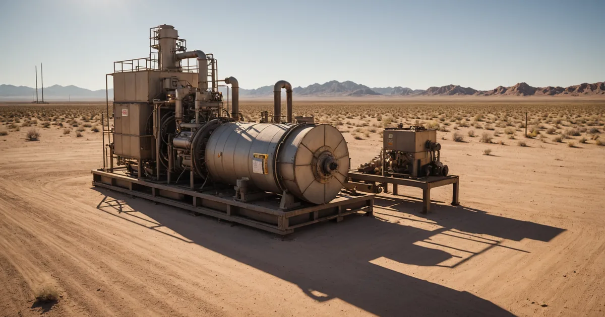
Being based in Phoenix has given us a specific education in what high ambient temperature does to equipment condition monitoring. When your summer baseline ambient is 43–46°C and outdoor equipment regularly sees enclosure temperatures above 60°C, thermal-based condition monitoring requires approaches that most PdM literature, written for temperate climates, doesn't fully address.
This isn't an abstract problem. Predictive maintenance baselines established in February become unreliable by July. Temperature-compensated models that work fine in Cleveland or Chicago behave poorly when the delta between design ambient and actual ambient hits 20°C and above. We've had to solve these problems because our early deployment work was in Arizona and the Sonoran Desert corridor, not in spite of it.
What 115°F ambient actually does to a motor
NEMA MG-1 motor ratings assume a 40°C (104°F) maximum ambient. That's already a design margin — most motors are designed to operate efficiently at somewhat lower ambient temperatures. When ambient reaches 43°C consistently, as it does during Phoenix summers, you've consumed that margin before the motor has done a single hour of work.
The practical consequences stack:
- Thermal headroom compression: A Class F insulation motor rated for a 155°C winding temperature operating in 40°C ambient has 115°C of rise budget. In 46°C ambient, that's reduced to 109°C — roughly a 6% reduction in thermal budget. That 6% doesn't sound alarming, but motors running near rated load in high ambient conditions are already consuming most of their rise budget. The cushion that normally absorbs a bearing friction increase or a cooling restriction disappears faster.
- Cooling fan inefficiency: TEFC motors depend on shaft-driven fans for cooling. Fan cooling efficiency is a function of the temperature differential between the motor frame and ambient air. In high ambient, that differential shrinks, and the same shaft speed delivers less effective cooling. You can see this in winding temperature rise rates — a motor that might take 90 minutes to reach thermal equilibrium in Phoenix winter may reach it in 60 minutes in July.
- Bearing grease degradation acceleration: This is the one most directly relevant to our work. Grease viscosity drops nonlinearly with temperature. A grease rated for 120°C service starts experiencing measurable viscosity thinning above 80°C in the bearing housing. In a Phoenix summer, a motor running at 80% load in direct solar exposure can see bearing housing temperatures in the 85–95°C range. At that temperature, the grease film that separates rolling elements from the raceway is significantly thinner than what the grease specification assumes, increasing metal-to-metal contact probability and accelerating surface fatigue progression.
The baseline drift problem
Most PdM programs establish their healthy baselines during initial commissioning — often in autumn or winter when desert ambient temperatures are moderate. Those baselines capture what "healthy operation" looks like at, say, 18°C ambient. When July arrives and ambient jumps to 46°C, every temperature-sensitive sensor on that asset shifts.
Motor winding temperature rises by 20–25°C, not because anything is wrong, but because ambient changed. Bearing housing temperature rises. Lubricant viscosity readings shift. On a thermal monitoring system with fixed alarm thresholds, this generates a wave of alarms in June that are entirely ambient-driven — not condition-driven. If the RE doesn't know to expect this, the first Phoenix summer after deployment can look like simultaneous degradation across the entire monitored fleet.
We've seen this happen at facilities that deployed monitoring systems during winter commissioning. The first summer produces a flood of alerts, the maintenance team investigates and finds nothing wrong, and the system gets a reputation as unreliable. The thresholds get raised. The following summer produces genuine failures that the raised thresholds miss. This is a predictable failure mode if you know to look for it, and an expensive surprise if you don't.
The mitigation is ambient temperature compensation built into the baseline model — not as a post-hoc correction but as a core feature of how baselines are stored and alarm thresholds are calculated. The question being asked shouldn't be "is this motor above its absolute temperature limit?" but "is this motor running hotter than expected at this ambient temperature, this load level, and this run duration?"
Grease selection and monitoring intervals in desert conditions
Grease interval recommendations from bearing manufacturers are given in operating hours at a specific temperature. SKF, NSK, and FAG all publish temperature correction factors for their regreasing intervals — typically a factor of roughly 0.5× for every 15°C above 70°C bearing operating temperature. What this means in practice: a bearing that might need regreasing every 2,000 hours at 60°C housing temperature should be regreased every 1,000 hours at 75°C, and every 500 hours at 90°C.
In Phoenix summer conditions, it's not unusual for medium-duty motors running in outdoor enclosures or poorly-ventilated mechanical rooms to reach 85–90°C bearing housing temperatures. At that temperature, the published 6-month or annual regreasing interval that the maintenance team has followed for years may be shortening the bearing life rather than protecting it, because grease is either hardening from oxidation at high temperature or thinning to the point of inadequate film thickness.
Acoustic emission monitoring is particularly well-suited to detecting this condition because AE picks up the ultrasonic signatures of metal-to-metal contact and surface fatigue at frequencies well above what accelerometers catch at early stages. A bearing with inadequate lubrication film shows elevated AE baseline levels before any detectable change appears in velocity or acceleration spectra. In desert conditions, where thermal-driven grease degradation is a primary bearing failure pathway, that early AE signal is often the best — and sometimes the only — leading indicator that grease replenishment is overdue.
Solar loading: the variable nobody models
There's a heat source in Arizona that most equipment protection models ignore entirely: direct solar irradiance. An outdoor motor or pump in Phoenix summer receives approximately 800–1,000 W/m² of solar load during peak hours. For a motor with an exposed surface area of roughly 0.5 m², that's 400–500 W of additional heat input that no cooling system was designed to handle.
The practical effect is significant. A motor rated for 40°C ambient in shade may be operating at an effective thermal load equivalent to 55–60°C ambient when operating under direct sun during summer afternoons. The motor's temperature sensors, if they exist, will reflect this. Any monitoring system that doesn't have context about whether the asset is sun-exposed versus shaded will interpret the solar-driven temperature rise as a condition change rather than an environmental condition.
We've addressed this in our modeling by including a solar exposure flag in asset configuration — essentially a metadata field that tells the model "this asset receives direct solar loading from approximately 10:00 to 16:00 MST and should apply a solar load correction during those hours." It's not a perfect correction, but it reduces the rate of solar-driven false alarms enough to matter.
What doesn't change
We're not saying that desert heat makes bearing degradation physics different. The failure modes are the same — surface fatigue, spalling, fretting, raceway indentation from overload. The bearing defect frequencies (BPFO, BPFI, BSF) are still calculable from geometry and shaft speed. The P-F interval from initial defect to functional failure still exists and can still be exploited.
What changes is the background against which those signals need to be interpreted. The noise floor is higher — thermally-driven vibration, grease behavior, and baseline shifts all add variability to the signal. The window between first detectable anomaly and actionable alert narrows because degradation can accelerate faster when thermal headroom is already consumed. And the seasonal variation in what "normal" looks like is larger, requiring either a seasonal baseline model or an ambient-compensated model that adapts continuously.
A specific scenario worth walking through
Consider a 75 kW cooling tower fan motor at an industrial facility in the East Valley — an outer suburb of Phoenix — running essentially continuously from April through October. The motor is TEFC, installed horizontally, in an outdoor equipment pad with partial shade from a corrugated metal roof but no enclosure. Ambient during peak summer: 44–47°C. The motor was commissioned in November, baseline established at 22°C ambient.
By June, winding temperature runs 35°C above the November baseline at comparable load. Bearing housing temperature is up 28°C from baseline. The raw temperature numbers look alarming against November thresholds. But both are within expected range once ambient compensation is applied — the motor is hot but healthy.
In late July, AE levels on the drive-end bearing begin a gradual rise — not dramatic, but trending upward at roughly 1.2 dB per week over four weeks. Simultaneously, lube oil analysis (monthly sample) shows a slight increase in iron particle count. The temperature trend, once ambient-compensated, shows the drive-end bearing housing running 4°C hotter than the model predicts for the operating conditions. None of these individually crosses an alarm threshold. Together, they form a consistent picture of early surface fatigue, probably on the outer race.
That's the scenario where multi-sensor correlation earns its keep. Any single sensor, read without context, is either alarming on ambient effects or missing the early degradation. The synthesis of AE trend, particulate count, and temperature residual (actual minus predicted) points clearly at a specific bearing that warrants inspection before the next monthly survey.
This is the work. It's not glamorous, and it's not automatic. But it's the difference between a PdM program that works in Phoenix and one that works in a catalog photo from a temperate climate manufacturing plant.